Draw a Circle Graphics3d Mathematica
Preface
This section is devoted to some aspets of qualitative analysis of first order differential equations in normal form. Other properties of the solution such equally premises, asymptotic expansions, stability, periodicity, etc., without explicitly solving the equation, volition be expoited later.
Render to calculating page for the kickoff form APMA0330
Return to computing page for the second course APMA0340
Return to Mathematica tutorial for the second course APMA0340
Return to the primary page for the course APMA0330
Render to the primary page for the form APMA0330
Return to the principal page for the course APMA0340
Return to Function I of the course APMA0330
Parametric Plots
A parametric equation defines a group of quantities as functions of one or more contained variables called parameters. Parametric equations are commonly used to express the coordinates of the points that brand up a geometric object such as a bend or surface, in which instance the equations are collectively called a parametric representation or parameterization (alternatively spelled equally parametrisation) of the object. Mathematica has a dedicated command for these purposes: ParametricPlot.
As it tin be seen, you can practically brandish whatsoever implicit role using the implicitplot command. Explicitly divers functions tin can be plotted using the regular Plot command.
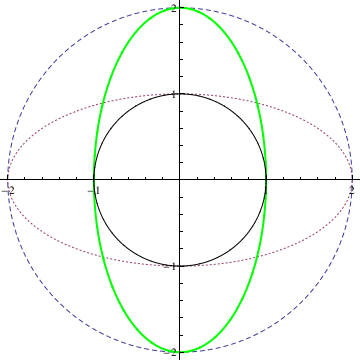 | ParametricPlot[{{2 Cos[t], 2 Sin[t]}, {2 Cos[t], Sin[t]}, {Cos[t], Plotlegent to identify equations in utilize. ParametricPlot[{{two Cos[t], 2 Sin[t]}, {2 Cos[t], Sin[t]}, {Cos[t], 2 Sin[t]}, {Cos[t], Sin[t]}}, {t, 0, two Pi}, PlotStyle -> {Dashed, Dashing[Tiny], Directive[Thick, Greenish], Blackness}, PlotLegends -> "Expressions"] |
You tin enjoy using a newer Mathematica parcel: NotebookEmbedder from Wolfram Cloud notebooks on websites
The input chemical element
Click the "Submit" button and the form-data volition be sent to Wolfram Cloud at this specific URL to generate a plot and return the event every bit a PNG paradigm".
Alternating view in blitheness form
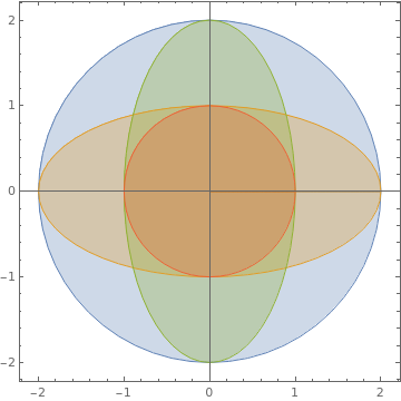 | Or you can brand a similar plot with overlapping regions: ParametricPlot[{{2 r Cos[t], 2 r Sin[t]}, {2 r Cos[t], r Sin[t]}, {r Cos[t], 2 r Sin[t]}, {r Cos[t], r Sin[t]}}, {t, 0, 2 Pi}, {r, 0, ane}, Mesh -> Faux] |
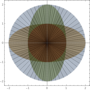 | Another option: ParametricPlot[{{two r Cos[t], 2 r Sin[t]}, {ii r Cos[t], r Sin[t]}, {r Cos[t], two r Sin[t]}, {r Cos[t], r Sin[t]}}, {t, 0, two Pi}, {r, 0, 1}, Mesh -> All] |
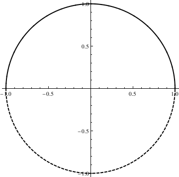 | ParametricPlot[{Cos[t], Sin[t]}, {t, 0, two Pi}, PlotStyle -> Directive[Thick, Black], Mesh -> {Range[0, 2 Pi, Pi]}, MeshShading -> {Dashed, {}}] |
We tin also plot a circle or ellipse using the following commands:
ten := Cos[t]; y := Sin[t] ParametricPlot[{x, y}, {t, 0, 2 Pi}] ParametricPlot[{2*x, y}, {t, 0, 2 Pi}]
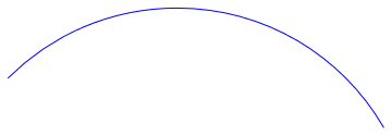 | Actually, in that location is a special command in Mathematica that can be used to plot circles and ellipses: Circle[{10,y},r] gives a circle of radius r centered at {x,y}. Circle[{x,y}] represents a circumvolve of radius one. Circumvolve[{x,y},{r_x , r_y}] gives an axis-aligned ellipse with semi-axes length r_x and r_y. Circumvolve[{10,y},..., {theta_1 , theta_2}] gives a a circular or ellipse arc from angle theta_1 to theta_2 Graphics[{Blue, Circle[{0, 1}, 2, {Pi/6, 3*Pi/4}]}] |
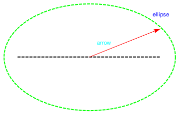 | R = Graphics[{Green, Thick, Dashed, Circle[{ane, 2}, {ane.two, 0.75}], {Bluish, Inset["ellipse", {two, 2.six}]}, {Black, Line[{{0, two}, {2, two}}]}}] |
To visualize spherical coordinates, use the following codes:
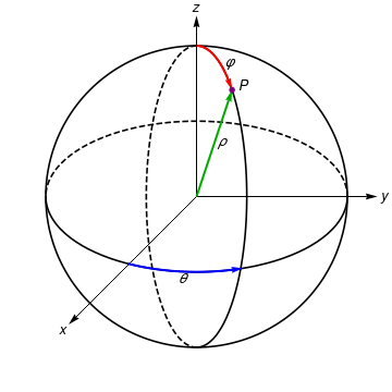 | circle[x_] = {Cos[x], Sin[x]}; ellipsePhi[x_, a_: - Pi/2] = {Cos[x - a]/three, Sin[x + a]}; ellipseTheta[x_, a_: 0] = {Cos[ten + a], Sin[-x - a]/ii}; ParametricPlot[circle[ten], {x, 0, ii Pi}, PlotStyle -> Black, Epilog -> Kickoff /@ {(*Ellipses*) ParametricPlot[{ellipsePhi[x], ellipsePhi[-x], ellipseTheta[-x], ellipseTheta[10]}, {10, 0, Pi}, PlotStyle -> {{Black, Dashed}, Black}],(*According axes*) Graphics[ Table[GeometricTransformation[{Arrowheads[0.03], Arrow[{{0, 0}, {one.2, 0}}]}, ReflectionMatrix[circle[ten]]], {ten, {Pi/2, -Pi/4, Pi/eight}}]], (*mark betoken,rho,phi& theta directions*) ParametricPlot[{ellipsePhi[ten, Pi/2], ellipseTheta[-x, 13 Pi/twenty]}, {10, 0, Pi/4}, PlotStyle -> {{Cherry, Thick}, {Blue, Thick}}] /. Line[x__] :> Sequence[Arrowheads[0.03], Arrow[10]], Graphics[{{Directive[Darker@Green, Thick], Arrowheads[0.03], Arrow[{{0, 0}, ellipsePhi[-iii Pi/4]}]}, {Directive[Purple], Disk[ellipsePhi[-3 Pi/4], 0.02]}}], (*text*) Graphics[{Text[Manner["x", Italic, Larger], ane.25 circumvolve[five Pi/4]], Text[Mode["y", Italic, Larger], 1.25 circle[0]], Text[Style["z", Italic, Larger], 1.25 circle[Pi/two]], Text[Way["\[Rho]", Italic, Larger], 0.four circle[four Pi/eleven]], Text[Style["\[CurlyPhi]", Italic, Larger], 1.1 ellipsePhi[Pi + Pi/5]], Text[Style["\[Theta]", Italic, Larger], ane.1 ellipseTheta[13 Pi/20 - Pi/viii]], Text[Way["P", Italic, Larger], 1.2 ellipsePhi[-3 Pi/four + Pi/24]]}] }, Axes -> False, PlotRange -> i.3 {{-ane, 1}, {-i, 1}} ] |
This culling solution has the advantage of beingness created using 3D directives. Every bit such, it was piece of cake to wrap within a Dispense and yous can drag it with your mouse to change the viewpoint:
Dispense[ Module[{x = Sin[\[Phi]] Cos[\[Theta]], y = Sin[\[Phi]] Sin[\[Theta]], z = Cos[\[Phi]]}, Show[ParametricPlot3D[{{Cos[t], Sin[t], 0}, {0, Sin[t], Cos[t]}, {Sin[t], 0, Cos[t]}}, {t, 0, ii \[Pi]}, PlotStyle -> Black, Boxed -> False, Axes -> False, AxesLabel -> {"10", "y", "z"}], ParametricPlot3D[0.5*{Cos[t], Sin[t], 0}, {t, 0, \[Theta]}], ParametricPlot3D[ RotationTransform[\[Theta], {0, 0, 1}][{Sin[t]/2, 0, Cos[t]/2}], {t, 0, \[Phi]}], Graphics3D[{{{Bluish, Thick, Pointer[{{0, 0, 0}, #}] & /@ {{1, 0, 0}, {0, one, 0}, {0, 0, 1}, {x, y, z}}}, {Opacity[0.i], Red, Polygon[{{0, 0, 0}, {10, y, 0}, {x, y, z}}], Green, Polygon[{{0, 0, 0}, {x, 0, 0}, {10, y, 0}}]}}, {Opacity[0.05], Sphere[{0, 0, 0}]}, {Text["O", {-.03, -.03, -.03}], Text["10", {1.i, 0, 0}], Text["Q", {10, y, 0}, {1, one}], Text["P", {x, y, z}, {0, -1}], Text["Y", {0, i.1, 0}], Text["Z", {0, 0, one.1}], Text["r", {x/2, y/2, 0}, {ane, ane}], Text["\[Theta]", {Cos[\[Theta]/2]/2, Sin[\[Theta]/2]/ii, 0}, {1, one}], Text["\[Phi]", RotationTransform[\[Theta], {0, 0, 1}][{Sin[\[Phi]/2]/ii, 0, Cos[\[Phi]/two]/2}], {ane, 1}]}}]]], {{\[Phi], \[Pi]/4}, 0.01, \[Pi]/two}, {{\[Theta], \[Pi]/4}, 0.01, two \[Pi]}]
Render to Mathematica folio
Return to the main page (APMA0330)
Return to the Part 1 (Plotting)
Return to the Part 2 (Start Order ODEs)
Return to the Part 3 (Numerical Methods)
Return to the Role four (Second and Higher Order ODEs)
Return to the Part 5 (Series and Recurrences)
Return to the Part 6 (Laplace Transform)
Render to the Part 7 (Boundary Value Problems)
Source: https://www.cfm.brown.edu/people/dobrush/am33/Mathematica/ch1/parametric.html
Post a Comment for "Draw a Circle Graphics3d Mathematica"